Persistence Images

Persistence Images were first introduced in Adams et al, 2017. Much of this work, and examples contained herein are inspired by the work of Obayashi and Hiraoka, 2017. Choices of weightings and general methods can be derived from Kusano, Fukumizu, and Yasuaki Hiraoka, 2016.

from itertools import product

import time
import numpy as np
from sklearn import datasets
from scipy.stats import multivariate_normal as mvn
import matplotlib.pyplot as plt

from ripser import Rips
from persim import PersistenceImager

The PersistenceImager() Class

# Printing a PersistenceImager() object will print its defining attributes
pimgr = PersistenceImager(pixel_size=0.2, birth_range=(0,1))
print(pimgr)

PersistenceImager(birth_range=(0.0, 1.0), pers_range=(0.0, 1.0), pixel_size=0.2, weight=persistence, weight_params={'n': 1.0}, kernel=gaussian, kernel_params={'sigma': [[1.0, 0.0], [0.0, 1.0]]})

# PersistenceImager() attributes can be adjusted at or after instantiation.
# Updating attributes of a PersistenceImager() object will automatically update all other dependent attributes.
pimgr.pixel_size = 0.1
pimgr.birth_range = (0, 2)
print(pimgr)
print(pimgr.resolution)

PersistenceImager(birth_range=(0.0, 2.0), pers_range=(0.0, 1.0), pixel_size=0.1, weight=persistence, weight_params={'n': 1.0}, kernel=gaussian, kernel_params={'sigma': [[1.0, 0.0], [0.0, 1.0]]})
(20, 10)

# The `fit()` method can be called on one or more (*,2) numpy arrays to automatically determine the miniumum birth and
# persistence ranges needed to capture all persistence pairs. The ranges and resolution are automatically adjusted to
# accomodate the specified pixel size.
pimgr = PersistenceImager(pixel_size=0.5)
pdgms = [np.array([[0.5, 0.8], [0.7, 2.2], [2.5, 4.0]]),
         np.array([[0.1, 0.2], [3.1, 3.3], [1.6, 2.9]]),
         np.array([[0.2, 1.5], [0.4, 0.6], [0.2, 2.6]])]
pimgr.fit(pdgms, skew=True)
print(pimgr)
print(pimgr.resolution)

PersistenceImager(birth_range=(0.1, 3.1), pers_range=(-8.326672684688674e-17, 2.5), pixel_size=0.5, weight=persistence, weight_params={'n': 1.0}, kernel=gaussian, kernel_params={'sigma': [[1.0, 0.0], [0.0, 1.0]]})
(6, 5)

# The `transform()` method can then be called on one or more (*,2) numpy arrays to generate persistence images from diagrams.
# The option `skew=True` specifies that the diagrams are currently in birth-death coordinates and must first be transformed
# to birth-persistence coordinates.
pimgs = pimgr.transform(pdgms, skew=True)
pimgs[0]

array([[0.03999068, 0.05688393, 0.06672051, 0.06341749, 0.04820814],
       [0.04506697, 0.06556791, 0.07809764, 0.07495246, 0.05730671],
       [0.04454486, 0.06674611, 0.08104366, 0.07869919, 0.06058808],
       [0.04113063, 0.0636504 , 0.07884635, 0.07747833, 0.06005714],
       [0.03625436, 0.05757744, 0.07242608, 0.07180125, 0.05593626],
       [0.02922239, 0.04712024, 0.05979033, 0.05956698, 0.04653357]])

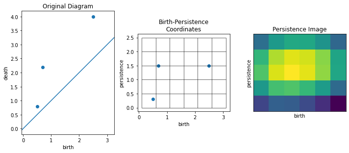
# The `plot_diagram()` and `plot_image()` methods can be used to visualize persistence diagrams and images
fig, axs = plt.subplots(1, 3, figsize=(10,5))

axs[0].set_title("Original Diagram")
pimgr.plot_diagram(pdgms[0], skew=False, ax=axs[0])

axs[1].set_title("Birth-Persistence\nCoordinates")
pimgr.plot_diagram(pdgms[0], skew=True, ax=axs[1])

axs[2].set_title("Persistence Image")
pimgr.plot_image(pimgs[0], ax=axs[2])

plt.tight_layout()

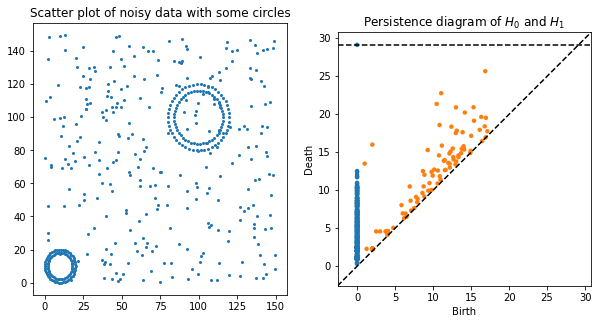
Generate a persistence diagram using Ripser

# lots of random noise and 2 circles
data = np.concatenate([150 * np.random.random((300,2)),
                       10 + 10 * datasets.make_circles(n_samples=100)[0],
                       100 + 20 * datasets.make_circles(n_samples=100)[0]])

rips = Rips()
dgms = rips.fit_transform(data)
H0_dgm = dgms[0]
H1_dgm = dgms[1]

plt.figure(figsize=(10,5))
plt.subplot(121)
plt.scatter(data[:,0], data[:,1], s=4)
plt.title("Scatter plot of noisy data with some circles")

plt.subplot(122)
rips.plot(dgms, legend=False, show=False)
plt.title("Persistence diagram of $H_0$ and $H_1$")
plt.show()

Rips(maxdim=1, thresh=inf, coeff=2, do_cocycles=False, n_perm = None, verbose=True)

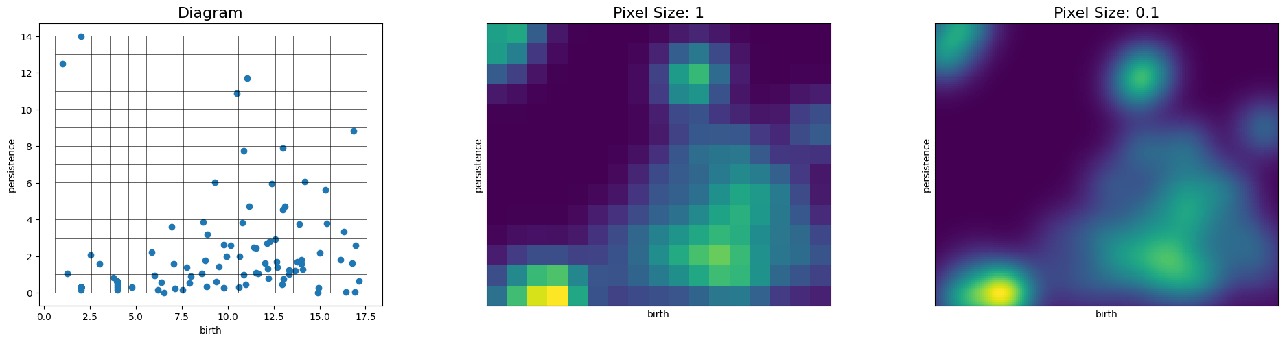
Modify the Image Resolution

# The resolution of the persistence image is adjusted by choosing the pixel size, given in the same units as the diagram
pimgr = PersistenceImager(pixel_size=1)
pimgr.fit(H1_dgm)

fig, axs = plt.subplots(1, 3, figsize=(20,5))
pimgr.plot_diagram(H1_dgm, skew=True, ax=axs[0])
axs[0].set_title('Diagram', fontsize=16)

pimgr.plot_image(pimgr.transform(H1_dgm), ax=axs[1])
axs[1].set_title('Pixel Size: 1', fontsize=16)

pimgr.pixel_size = 0.1
pimgr.plot_image(pimgr.transform(H1_dgm), ax=axs[2])
axs[2].set_title('Pixel Size: 0.1', fontsize=16)

plt.tight_layout()

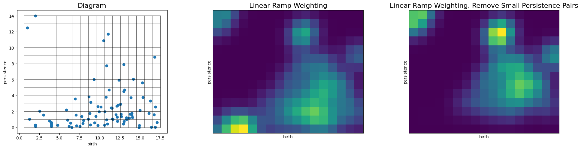
Modify the Weight function and parameters

# We first import one of the implemented weighting functions, a peicewise linear ramp
from persim.images_weights import linear_ramp

pimgr.pixel_size = 1
pimgr.weight = linear_ramp
pimgr.weight_params = {'low':0.0, 'high':1.0, 'start':0.0, 'end':10.0}

fig, axs = plt.subplots(1, 3, figsize=(20,5))
pimgr.plot_diagram(H1_dgm, skew=True, ax=axs[0])
axs[0].set_title('Diagram', fontsize=16)

pimgr.plot_image(pimgr.transform(H1_dgm), ax=axs[1])
axs[1].set_title('Linear Ramp Weighting', fontsize=16)

pimgr.weight_params = {'low':0.0, 'high':1.0, 'start':2.0, 'end':10.0}
pimgr.plot_image(pimgr.transform(H1_dgm), ax=axs[2])
axs[2].set_title('Linear Ramp Weighting, Remove Small Persistence Pairs', fontsize=16)

plt.tight_layout()

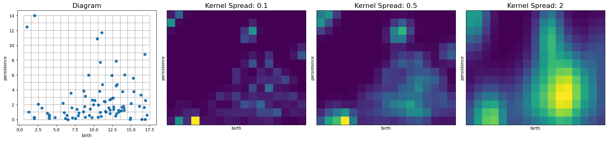
Modify the Persistence Pair Kernel

Reduce the standard deviate of the isotropic Gaussian kernel used.

# For the default bivariate normal Gaussian kernel, the parameter controlling the spread (sigma) may be specified
# either by a float or a 2x2 covariance matrix
pimgr = PersistenceImager(pixel_size=1)
pimgr.fit(H1_dgm)

fig, axs = plt.subplots(1, 4, figsize=(20,5))
pimgr.kernel_params = {'sigma': .1}
pimgr.plot_diagram(H1_dgm, skew=True, ax=axs[0])
axs[0].set_title('Diagram', fontsize=16)

pimgr.kernel_params = {'sigma': 0.1}
pimgr.plot_image(pimgr.transform(H1_dgm), ax=axs[1])
axs[1].set_title('Kernel Spread: 0.1', fontsize=16)

pimgr.kernel_params = {'sigma': .5}
pimgr.plot_image(pimgr.transform(H1_dgm), ax=axs[2])
axs[2].set_title('Kernel Spread: 0.5', fontsize=16)

# Non-isotropic, standard bivariate Gaussian with greater spread along the persistence axis
pimgr.kernel_params = {'sigma': np.array([[1, 0],[0, 6]])}
pimgr.plot_image(pimgr.transform(H1_dgm), ax=axs[3])
axs[3].set_title('Kernel Spread: 2', fontsize=16)

plt.tight_layout()

# A valid kernel is a python function of the form kernel(x, y, mu=(birth, persistence), **kwargs) defining a
# cumulative distribution function such that kernel(x, y) = P(X <= x, Y <=y), where x and y are numpy arrays of equal length.
# The required parameter mu defines the dependance of the kernel on the location of a persistence pair and is usually
# taken to be the mean of the probability distribution function associated to kernel CDF.

# Example of a custom kernel which defines the cumulative distribution function for the uniform probability density
# with value 1/(width*height) over the region [mu[0]-width/2, mu[0]+width/2] x [mu[1]-height/2, mu[1]+height/2]
def uniform_kernel(x, y, mu=None, width=1, height=1):
    w1 = np.maximum(x - (mu[0] - width/2), 0)
    h1 = np.maximum(y - (mu[1] - height/2), 0)

    w = np.minimum(w1, width)
    h = np.minimum(h1, height)

    return w*h / (width*height)

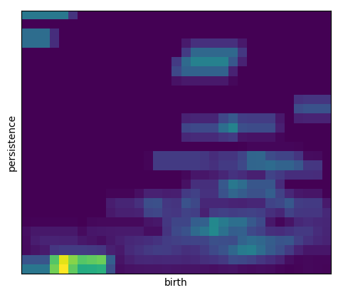
# Construct a PersistenceImager() object that uses the uniform distribution kernel supported on a rectangular region
pimgr = PersistenceImager(pixel_size=.5, kernel=uniform_kernel, kernel_params={'width': 3, 'height': 1})
pimgr.fit(H1_dgm)
pimgr.plot_image(pimgr.transform(H1_dgm))

<AxesSubplot:xlabel='birth', ylabel='persistence'>

Parallelization

# For diagrams with small numbers of persistence pairs, overhead costs may not justify parallelization
# Also, initial run of job in parallel is very costly. Run twice to see speed gains.
import time
num_diagrams = 100
min_pairs = 50
max_pairs = 100

pimgr = PersistenceImager()
dgms = [np.random.rand(np.random.randint(min_pairs, max_pairs), 2) for _ in range(num_diagrams)]

pimgr.fit(dgms)

start_time = time.time()
pimgr.transform(dgms)
print("Execution time in serial: %g sec." % (time.time() - start_time))

start_time = time.time()
pimgr.transform(dgms, n_jobs=-1)
print("Execution time in parallel: %g sec." % (time.time() - start_time))

Execution time in serial: 0.159616 sec.
Execution time in parallel: 0.143826 sec.

# For larger diagrams, speed up can be significant
import time
num_diagrams = 100
min_pairs = 500
max_pairs = 1000

pimgr = PersistenceImager()
dgms = [np.random.rand(np.random.randint(min_pairs, max_pairs), 2) for _ in range(num_diagrams)]

pimgr.fit(dgms)

start_time = time.time()
pimgr.transform(dgms)
print("Execution time in serial: %g sec." % (time.time() - start_time))

start_time = time.time()
pimgr.transform(dgms, n_jobs=-1)
print("Execution time in parallel: %g sec." % (time.time() - start_time))

Execution time in serial: 1.51495 sec.
Execution time in parallel: 0.442808 sec.