Distinguishing spheres using persistence landscapes
In this notebook, we will highlight some basic functionality of the PersLandscapeApprox class and how it can be used to perform a permutation test through a simple experiment.
The experiment is to determine if persistent homology can distinguish between spheres of different dimensions. Here we restrict to differentiating \(S^2\) from \(S^3\). We will further restrict ourselves to persistent homology in degree one (but one can use all relevant homological degrees as well). A priori, we would not expect this to be an effective discriminator, since the ordinary first homology of both spheres is trivial. Note that this is a simplified version of the experiment from Bubenik and Dlotko’s A persistence landscapes toolbox for topological statistics [1].
In detail:
Repeat the following
num_runs = 100times:Sample
num_pts = 100points from the 2-sphere and the 3-sphere. We rescale the spheres so the average distance between the points on each sphere is approximately 1.Compute the VR persistent homology (using
ripser) and compute the associated landscapes. Store each of these landscapes.Compute the average landscape for \(S^2\) and \(S^3\). Take the difference of these two, and finally compute its supremum norm. This yields a real number; call it
significance.
We have thus established a baseline significance and we will see if the labelling of landscapes by dimension of their underlying sphere is significant as follows. Repeat the following
num_perms = 1000times:Using the stored landscapes, randomly label half as belonging to class A and the other half as class B.
Compute the average landscape of class A, the average landscape of class B. Compute their difference and its sup norm.
If the sup norm of a shuffled set of labels is larger than
significance, then we say that particular shuffling of labels was significant. If the sup norm is smaller thansignificance, then that labelling was not significant.Take the total number of significant labellings and divide by
num_permsto get the p-value of this permutation test. If this p-value is less than some threshold (say 0.05), then we accept the hypothesis that the labelling based on the sphere’s dimension is significant. Otherwise, we reject.
[1]:
import random

from ripser import ripser
from persim.landscapes import (
    PersLandscapeApprox,
    average_approx,
    snap_pl,
    plot_landscape,
    plot_landscape_simple,
)
from tadasets import dsphere
The aforementioned parameters taken from [1]. We modify these parameters below to speed up the computation.
[2]:
num_pts = 100
num_runs = 100
num_perms = 1000
Establish the baseline
The following cell samples the points, computes the persistent homology and the landscapes. Depending on the above parameters, it could take a while.
We also scale the points according to the average distance between points on \(S^2\) and \(S^3\), respectively (given here https://math.stackexchange.com/q/2366580/22378). One could compute the actual distance on each run and normalize by that number, but that is more computationally intensive and isn’t needed for this simple exercise. Note that tadasets implementation of dsphere samples points uniformly.
[3]:
sph2_pl1 = []
sph3_pl1 = []

for _ in range(num_runs):
    sph2 = dsphere(n=num_pts, d=2) / 1.3333  # sample points, scaling appropriately
    sph2_dgm = ripser(sph2, maxdim=2)["dgms"]  # compute PH0, PH1, PH2
    sph2_pl = PersLandscapeApprox(
        dgms=sph2_dgm, hom_deg=1
    )  # compute persistence landscape
    sph2_pl1.append(sph2_pl)

    sph3 = dsphere(n=num_pts, d=3) / 1.3581  # sample points, scaling appropriately
    sph3_dgm = ripser(sph3, maxdim=2)["dgms"]  # compute PH0, PH1, PH2
    sph3_pl = PersLandscapeApprox(
        dgms=sph3_dgm, hom_deg=1
    )  # compute persistence landscape
    sph3_pl1.append(sph3_pl)
We now compute the average landscape of each list of landscapes. This can be done manually, but there is a method average_approx that will snap each entry to a common grid and compute the average efficiently.
[4]:
avg_sph2 = average_approx(sph2_pl1)
avg_sph3 = average_approx(sph3_pl1)
print(avg_sph2, "\n")
print(avg_sph3)
Approximate persistence landscape in homological degree 1 on grid from 0.0718967542052269 to 0.8019469380378723 with 500 steps

Approximate persistence landscape in homological degree 1 on grid from 0.12950880825519562 to 0.8291281461715698 with 500 steps
Each of these average landscapes have been computed, but are on different grids, so we must first snapt them to a common grid before taking their difference.
[5]:
[avg_sph2_snapped, avg_sph3_snapped] = snap_pl([avg_sph2, avg_sph3])
true_diff_pl = avg_sph2_snapped - avg_sph3_snapped
significance = true_diff_pl.sup_norm()

print(f"The threshold for significance is {significance}.")
The threshold for significance is 0.06032077519378484.
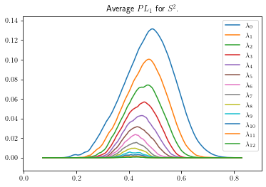
Can we see the differences qualititatively?
[6]:
# view figures in notebook
# %matplotlib inline

plot_landscape_simple(
    avg_sph2_snapped, title="Average $PL_1$ for $S^2$.", depth_range=range(13)
)
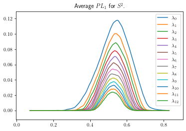
[7]:
plot_landscape_simple(
    avg_sph3_snapped, title="Average $PL_1$ for $S^2$.", depth_range=range(13)
)
[8]:
plot_landscape_simple(
    true_diff_pl, title="Difference of average PLs", depth_range=range(13)
)
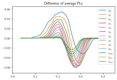
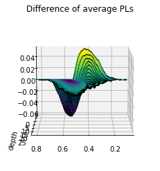
The last figure has a lot going on. We can try the 3d plotting method as well to see more depth. This method is slower, and better used for final figure and not exploration.
[9]:
plot_landscape(true_diff_pl, title="Difference of average PLs")
Perform the permutation test
[10]:
comb_pl = sph2_pl1 + sph3_pl1
sig_count = 0

for shuffle in range(num_perms):
    A_indices = random.sample(range(2 * num_runs), num_runs)
    B_indices = [_ for _ in range(2 * num_runs) if _ not in A_indices]

    A_pl = [comb_pl[i] for i in A_indices]
    B_pl = [comb_pl[j] for j in B_indices]

    A_avg = average_approx(A_pl)
    B_avg = average_approx(B_pl)
    [A_avg_sn, B_avg_sn] = snap_pl([A_avg, B_avg])

    shuff_diff = A_avg_sn - B_avg_sn
    if shuff_diff.sup_norm() >= significance:
        sig_count += 1

pval = sig_count / num_perms

print(
    f"There were {sig_count} shuffles out of {num_perms} that",
    "were more significant than the true labelling. Thus, the",
    f"p-value is {pval}.",
)
There were 0 shuffles out of 1000 that were more significant than the true labelling. Thus, the p-value is 0.0.
So there wasn’t a single run of our experiment that resulted in a more significant labelling than the original one based on each sphere’s dimension! Therefore we conclude there is a strong statistical difference between the persistence landscapes in degree one for \(S^2\) and \(S^3\).
References
[1] Bubenik, P. & Dlotko, P. A persistence landscapes toolbox for topological statistics. Journal of Symbolic Computation 78, 91–114 (2017).