Persistence Landscapes and Machine Learning

This notebook gives usage examples for the persistence landscape functionality in persim and how they connect with other tools from scikit-learn. We will construct persistence landscapes for two different datasets (a sphere and a torus), plot them in comparison with each other, and use statistical learning tools to classify the two types of landscapes.

Example Plots for Torus vs Sphere

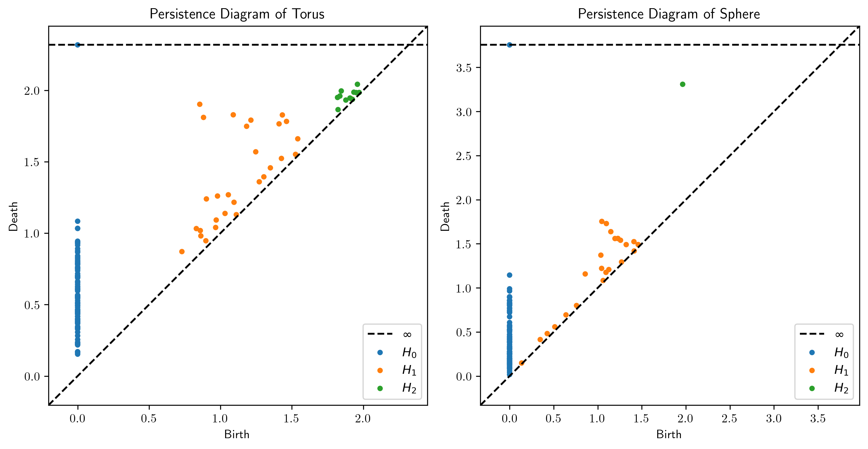
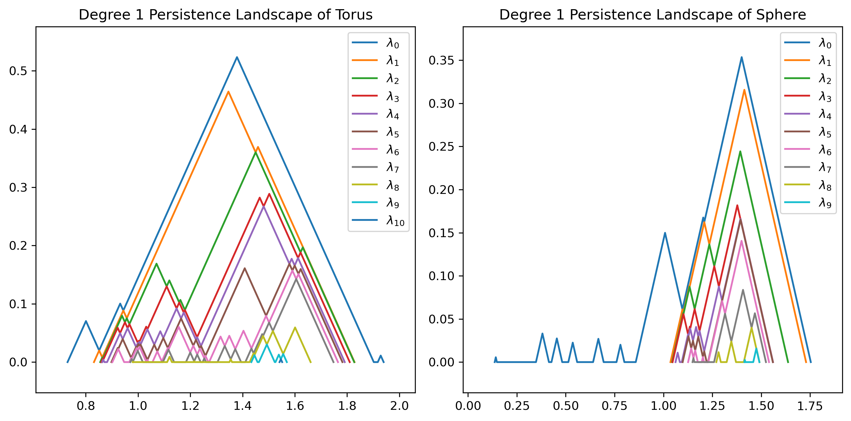
In this section, we plot persistence diagrams and persistence landscapes for a torus and a sphere to give an example of the data types and analysis results we will use in the larger-scale classification problem.

# Import general utilities
import numpy as np
import matplotlib
import matplotlib.pyplot as plt

# Import TDA utilities
from ripser import Rips
from tadasets import torus, sphere
from persim.landscapes import PersLandscapeExact
from persim.landscapes import plot_landscape_simple
from persim.landscapes import PersistenceLandscaper
from persim import plot_diagrams

# Import Scikit-Learn tools
from sklearn.decomposition import PCA
from sklearn import svm
from sklearn import metrics
from sklearn.model_selection import train_test_split

# Instantiate datasets
data_torus = torus(n=100, c=2, a=1)
data_sphere = sphere(n=100, r=2)

# Instantiate Vietoris-Rips solver
rips = Rips(maxdim = 2)

Rips(maxdim=2, thresh=inf, coeff=2, do_cocycles=False, n_perm = None, verbose=True)

# Compute persistence diagrams
dgms_torus = rips.fit_transform(data_torus)
dgms_sphere = rips.fit_transform(data_sphere)

# Plot persistence diagrams
fig, axs = plt.subplots(1, 2, dpi=300)
fig.set_size_inches(10, 5)

plot_diagrams(dgms_torus, title="Persistence Diagram of Torus", ax=axs[0])

plot_diagrams(dgms_sphere, title="Persistence Diagram of Sphere", ax=axs[1])

fig.tight_layout()

# Plot persistence landscapes
fig, axs = plt.subplots(1, 2, dpi=300)
fig.set_size_inches(10, 5)

plot_landscape_simple(PersLandscapeExact(dgms_torus, hom_deg=1),
                             title="Degree 1 Persistence Landscape of Torus", ax=axs[0])

plot_landscape_simple(PersLandscapeExact(dgms_sphere, hom_deg=1),
                            title="Degree 1 Persistence Landscape of Sphere", ax=axs[1])

fig.tight_layout()

PCA and Classification

In this section, we implement principal component analysis and support vector classification to attempt to classify persistence landscapes generated from a torus and persistence landscapes generated from a sphere. This section is a basic implementation and can be optimized in many ways, a couple possible methods are described in the next section.

# Compute multiple persistence landscapes

landscapes_torus = []
landscapes_sphere = []

for i in range(100):
    # Resample data
    _data_torus = torus(n=100, c=2, a=1)
    _data_sphere = sphere(n=100, r=2)

    # Compute persistence diagrams
    dgm_torus = rips.fit_transform(_data_torus)

    # Instantiate persistence landscape transformer
    torus_landscaper = PersistenceLandscaper(hom_deg=1, start=0, stop=2.0, num_steps=500, flatten=True)

    # Compute flattened persistence landscape
    torus_flat = torus_landscaper.fit_transform(dgm_torus)

    landscapes_torus.append(torus_flat)

    # Compute persistence diagrams
    dgm_sphere = rips.fit_transform(_data_sphere)

    # Instantiate persistence landscape transformer
    sphere_landscaper = PersistenceLandscaper(hom_deg=1, start=0, stop=2.0, num_steps=500, flatten=True)

    # Compute flattened persistence landscape
    sphere_flat = sphere_landscaper.fit_transform(dgm_sphere)

    landscapes_sphere.append(sphere_flat)

landscapes_torus = np.array(landscapes_torus, dtype=object)
landscapes_sphere = np.array(landscapes_sphere, dtype=object)
print('Torus:', np.shape(landscapes_torus))
print('Sphere:', np.shape(landscapes_sphere))

Torus: (100,)
Sphere: (100,)

In order to make this data interpretable by a PCA solver, we need a (N, M) matrix. As seen in the above print statements, each entry in landscapes_sphere and landscapes_torus are not the same length! This is because there may be different amounts of \(\lambda_k\) functions for each resampling of the data.

To fix this, we can use zero padding to embed the arrays above in a larger (100, w) matrix, where w is the maximal length of a flattened landscape.

# Find maximal length
u = np.max([len(a) for a in landscapes_torus])
v = np.max([len(a) for a in landscapes_sphere])

w = np.max([u,v])

# Instantiate zero-padded arrays
ls_torus = np.zeros((100, w))
ls_sphere = np.zeros((100, w))

# Populate arrays
for i in range(len(landscapes_torus)):
    ls_torus[i, 0:len(landscapes_torus[i])] = landscapes_torus[i]
    ls_sphere[i, 0:len(landscapes_sphere[i])] = landscapes_sphere[i]


print('Torus:', ls_torus.shape)
print('Sphere:', ls_sphere.shape)

Torus: (100, 8500)
Sphere: (100, 8500)

Now, we have a matrix that we can apply PCA to!

# Instantiate PCA solver
pca_torus = PCA(n_components=2)

# Compute PCA
pca_torus.fit_transform(ls_torus)

# Define components
comp_torus = pca_torus.components_

# Instantiate PCA solver
pca_sphere = PCA(n_components=2)

# Compute PCA
pca_sphere.fit_transform(ls_sphere)

# Define components
comp_sphere = pca_sphere.components_

We can understand the results of PCA using the singular values computed in the PCA process.

print('Singular values for torus dataset:', pca_torus.singular_values_)
print('Singular values for sphere dataset:', pca_sphere.singular_values_)

Singular values for torus dataset: [11.3183319  10.27267007]
Singular values for sphere dataset: [11.47153282 11.19259913]

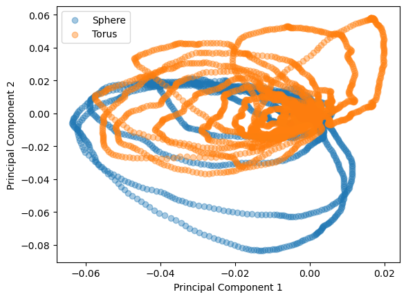
# Plot projection of data onto the first two principal components
plt.figure()
plt.scatter(comp_sphere[0], comp_sphere[1], label='Sphere', alpha=0.4)
plt.scatter(comp_torus[0], comp_torus[1], label='Torus', alpha=0.4)
plt.xlabel('Principal Component 1')
plt.ylabel('Principal Component 2')
plt.legend()

<matplotlib.legend.Legend at 0x7f34a0694d90>

We now want to use a support vector classifier to classify between landscapes computed on a torus and landscapes computed on a sphere. To do so, we need a list of points \(L\) and a function \(f: L \to \{0, 1\}\) so that \(f \equiv 0\) for torus landscapes and \(f \equiv 1\) on sphere landscapes.

# Produce lists of points
pts_torus = [[comp_torus[0,i], comp_torus[1,i]] for i in range(len(comp_torus[0]))]
pts_sphere = [[comp_sphere[0,i], comp_sphere[1,i]] for i in range(len(comp_sphere[0]))]

# Instantiate indicator functions
chi_torus = np.zeros(len(pts_torus))
chi_sphere = np.ones(len(pts_sphere))

# Produce final list of points
pts = []

for p in pts_torus:
    pts.append(p)

for p in pts_sphere:
    pts.append(p)

pts = np.array(pts)

# Append indicator functions
chi = np.hstack((chi_torus, chi_sphere))

To train the model, we use a simple 80-20 train/test split. We can improve this training schema by using cross-validation or other similar techniques.

# Split points and indicator arrays
P_train, P_test, c_train, c_test = train_test_split(pts, chi, train_size=.8)

# Instantiate support vector classifier
clf = svm.SVC()

# Fit model
clf.fit(P_train, c_train)

# Evaluate model performance using accuracy between ground truth data and predicted data
print(f'Model accuracy: {metrics.accuracy_score(c_test, clf.predict(P_test)):.2f}')

Model accuracy: 0.59

The model currently is not particularly accurate, but better than guessing! Hopefully, this gives a baseline implementation that statistical learning experts can improve with more robust models.

Improving Classification Accuracy

In this section, we go over some methods that can be implemented to improve the accuracy of the classification presented above.

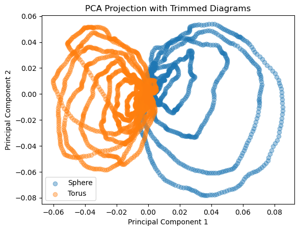
First, we try deleting highly persistent classes to point the model at smaller-scale data, encouraging geometric properties to inform the model.

Second, we try adding more principal components to the model to capture more degrees of freedom in the initial data.

Spoiler alert: the first approach does not show a significant improvement in this use case, but may be useful for other datasets. The second approach shows a minor improvement, hinting that the first two principal components may not capture enough data for classification purposes.

# Delete highly persistent landscapes

# Instantiate trimmed arrays
ls_torus_trim = ls_torus
ls_sphere_trim = ls_sphere

# Trim arrays
for i in range(len(landscapes_torus)):
    ls_torus_trim[i, 0:1000] = np.zeros((1000,))
    ls_sphere_trim[i, 0:1000] = np.zeros((1000,))


print('Torus:', ls_torus_trim.shape)
print('Sphere:', ls_sphere_trim.shape)

Torus: (100, 8500)
Sphere: (100, 8500)

# Instantiate PCA solver
pca_torus_trim = PCA(n_components=2)

# Compute PCA
pca_torus_trim.fit_transform(ls_torus_trim)

# Define components
comp_torus_trim = pca_torus_trim.components_

# Instantiate PCA solver
pca_sphere_trim = PCA(n_components=2)

# Compute PCA
pca_sphere_trim.fit_transform(ls_sphere_trim)

# Define components
comp_sphere_trim = pca_sphere_trim.components_

# Plot projection of data onto the first two principal components
plt.figure()
plt.scatter(comp_sphere_trim[0], comp_sphere_trim[1], label='Sphere', alpha=0.4)
plt.scatter(comp_torus_trim[0], comp_torus_trim[1], label='Torus', alpha=0.4)
plt.xlabel('Principal Component 1')
plt.ylabel('Principal Component 2')
plt.title('PCA Projection with Trimmed Diagrams')
plt.legend()

<matplotlib.legend.Legend at 0x7f34a093c700>

We now want to use a support vector classifier to classify between landscapes computed on a torus and landscapes computed on a sphere. To do so, we need a list of points \(L\) and a function \(f: L \to \{0, 1\}\) so that \(f \equiv 0\) for torus landscapes and \(f \equiv 1\) on sphere landscapes.

# Produce lists of points
pts_torus = [[comp_torus[0,i], comp_torus[1,i]] for i in range(len(comp_torus[0]))]
pts_sphere = [[comp_sphere[0,i], comp_sphere[1,i]] for i in range(len(comp_sphere[0]))]

# Instantiate indicator functions
chi_torus = np.zeros(len(pts_torus))
chi_sphere = np.ones(len(pts_sphere))

# Produce final list of points
pts = []

for p in pts_torus:
    pts.append(p)

for p in pts_sphere:
    pts.append(p)

pts = np.array(pts)

# Append indicator functions
chi = np.hstack((chi_torus, chi_sphere))

To train the model, we use a simple 80-20 train/test split. In practice, this can be improved by using cross-validation or other such techniques.

# Produce lists of points
pts_torus_trim = [[comp_torus_trim[0,i], comp_torus_trim[1,i]] for i in range(len(comp_torus_trim[0]))]
pts_sphere_trim = [[comp_sphere_trim[0,i], comp_sphere_trim[1,i]] for i in range(len(comp_sphere_trim[0]))]

# Instantiate indicator functions
chi_torus_trim = np.zeros(len(pts_torus_trim))
chi_sphere_trim = np.ones(len(pts_sphere_trim))

# Produce final list of points
pts_trim = []

for p in pts_torus_trim:
    pts_trim.append(p)

for p in pts_sphere_trim:
    pts_trim.append(p)

pts_trim = np.array(pts_trim)

# Append indicator functions
chi_trim = np.hstack((chi_torus_trim, chi_sphere_trim))

# Split points and indicator arrays
P_train_trim, P_test_trim, c_train_trim, c_test_trim = train_test_split(pts_trim, chi_trim, train_size=.8)

# Instantiate support vector classifier
clf_trim = svm.SVC()

# Fit model
clf_trim.fit(P_train_trim, c_train_trim)

# Evaluate model performance using accuracy between ground truth data and predicted data
print(f'Model accuracy: {metrics.accuracy_score(c_test_trim, clf_trim.predict(P_test_trim)):.2f}')

Model accuracy: 0.58

Improving Classification Accuracy

In this section, we go over some methods to improve the accuracy of the classification presented above. These methods include deleting highly persistent classes to identify significant differences in the data and using multicomponent PCA projections to capture more degrees of freedom in the initial data.

# Try multicomponent PCA

# Instantiate multicomponent PCA solver
pca_torus_mcomp = PCA(n_components=6)

# Compute PCA
pca_torus_mcomp.fit_transform(ls_torus)

# Define components
comp_torus_mcomp = pca_torus_mcomp.components_

# Instantiate PCA solver
pca_sphere_mcomp = PCA(n_components=6)

# Compute PCA
pca_sphere_mcomp.fit_transform(ls_sphere)

# Define components
comp_sphere_mcomp = pca_sphere_mcomp.components_


# Produce lists of points
pts_torus_mcomp = [[comp_torus_mcomp[j,i] for j in range(6)] for i in range(len(comp_torus_mcomp[0]))]
pts_sphere_mcomp = [[comp_sphere_mcomp[j,i] for j in range(6)] for i in range(len(comp_sphere_mcomp[0]))]

# Instantiate indicator functions
chi_torus_mcomp = np.zeros(len(pts_torus_mcomp))
chi_sphere_mcomp = np.ones(len(pts_sphere_mcomp))

# Produce final list of points
pts_mcomp = []

for p in pts_torus_mcomp:
    pts_mcomp.append(p)

for p in pts_sphere_mcomp:
    pts_mcomp.append(p)

pts_mcomp = np.array(pts_mcomp)

# Append indicator functions
chi_mcomp = np.hstack((chi_torus_mcomp, chi_sphere_mcomp))

# Split points and indicator arrays
P_train_mcomp, P_test_mcomp, c_train_mcomp, c_test_mcomp = train_test_split(pts_mcomp, chi_mcomp, train_size=.8)

# Instantiate support vector classifier
clf_mcomp = svm.SVC()

# Fit model
clf_mcomp.fit(P_train_mcomp, c_train_mcomp)

# Evaluate model performance using accuracy between ground truth data and predicted data
print(f'Model accuracy: {metrics.accuracy_score(c_test_mcomp, clf_mcomp.predict(P_test_mcomp)):.2f}')

Model accuracy: 0.61